CO oxidation in a reactor
Here, we will consider the CO oxidation reaction on neat Pd and an AuPd alloy, using DFT data from Tiburski et al. 1 Three elementary steps are considered, accounting for reversible adsorption of CO and dissociative adsorption of oxygen, and irreversible conversion of adsorbed CO and oxygen to carbon dioxide. Where s represents a free catalyst site:
Creating an input file
The previous example described the components required to specify an input file. Here, we will create two input files, one for Pd111 and one for AuPd. In this example, we will use the harmonic approximation (only vibrational free energy contributions) for adsorbate states, and the ideal gas approximation (vibrational, rotational and translational free energy contributions) for gas states. We will compute the energy of the TS state using the scaling relation for CO oxidation given in Falsig et al. 2 (more on this later). We will read the electronic energies calculated using DFT from OUTCAR files from VASP and the frequencies from vib.log files created using ASE and VASP. We will let PyCatKin obtain the necessary information about the gas molecules (mass, inertia and shape) from their respective atoms objects using ASE. In this example, the data is stored in a directory called data, with subdirectories for each state.
With this information, we can specify the states which include the clean surface (s), adsorbed CO (sCO) and O (sO) and gaseous CO, O2 and CO2:
{
    "states":
    {
        "s":
        {
            "state_type": "surface",
            "path": "data/Pd111"
        },
        "sCO":
        {
            "state_type": "adsorbate",
            "path": "data/CO.Pd111"
        },
        "sO":
        {
            "state_type": "adsorbate",
            "path": "data/O.Pd111"
        },
        "CO":
        {
            "state_type": "gas",
            "sigma": 1,
            "path": "data/CO"
        },
        "O2":
        {
            "state_type": "gas",
            "sigma": 2,
            "path": "data/O2"
        },
        "CO2":
        {
            "state_type": "gas",
            "sigma": 2,
            "path": "data/CO2"
        }
    },...
}
The above specifies the Pd111 states. The input file for AuPd will be equivalent but with the paths set to “data/AuPd”, “data/CO.AuPd” and “data/O.AuPd” for the adsorbates.
Note that we have not defined a transition state for the reaction. Here, we will introduce a ScalingState class state using the keyword scaling relation states and call it SRTS. Scaling relation states are defined by providing a dictionary of scaling_coeffs, the gradient and intercept of the scaling relation and a dictionary of scaling_reactions, the reactions that specify the binding energies the scaling relation depends on. Note that the Falsig scaling relation depends on the binding energy of O, but we will define the adsorption reaction for O2, which will lead to two bound oxygen atoms; thus, we need to specify a multiplicity of 0.5:
{
   "scaling relation states":
    {
        "SRTS":
        {
            "state_type": "TS",
            "scaling_coeffs":
            {
                "gradient": 0.7,
                "intercept": 0.02
            },
            "scaling_reactions":
            {
                "CO":
                {
                    "reaction": "CO_ads",
                    "multiplicity": 1.0
                },
                "O":
                {
                    "reaction": "O2_ads",
                    "multiplicity": 0.5
                }
            },
            "dereference": true,
            "use_descriptor_as_reactant": true
        }
    },...
}
The setting dereference=True is required in this example because we will need to subtract the absolute energies of the transition state and adsorbates to calculate the reaction barrier. The setting use_descriptor_as_reactant=True tells the code to use define the entropy of the transition state using the entropy of the states in the scaling_reactions. This works in this case because the scaling relation is defined in terms of the same species as the reaction step it specifies. In general, however, it is best to specify the entropy separately and leave this setting at its default value of False.
Next, we will specify the reactions. The chosen CO oxidation mechanism is very simple, consisting of barrierless adsorption reactions for CO and O2, with O2 adsorbing dissociatively, and an Arrhenius oxidation reaction to produce CO2, which is assumed to desorb spontaneously and irreversibly. Thus the reactions section of our input file:
{
    "reactions":
    {
        "CO_ads":
        {
            "reac_type": "adsorption",
            "area": 1.3e-19,
            "reactants": ["CO", "s"],
            "TS": null,
            "products": ["sCO"]
        },
        "O2_ads":
        {
            "reac_type": "adsorption",
            "area": 1.3e-19,
            "reactants": ["O2", "s", "s"],
            "TS": null,
            "products": ["sO", "sO"]
        },
        "CO_ox":
        {
            "reac_type": "Arrhenius",
            "area": 5.1e-19,
            "reactants": ["sCO", "sO"],
            "TS": ["SRTS"],
            "products": ["s", "s", "CO2"],
            "reversible": false
        }
    },...
}
Here, we will use a reactor of the type CSTReactor (continuously stirred tank reactor), wherein the boundary conditions (gas concentrations) are the reactor inflow and we study both surface kinetics and mass transport effects. The CSTReactor is defined by its residence_time (the volume divided by the flow rate), volume and total catalyst_area:
{
    "reactor":
    {
        "CSTReactor":
        {
            "residence_time": 4.5,
            "volume": 180.0e-9,
            "catalyst_area": 3.82e-09
        }
    },...
}
If the residence time is unknown, the flow rate can be specified instead. The volume and catalyst_area are used to scale up the surface kinetics from a per-site basis to a per-reactor basis.
Now, we can specify the system. The options provided to system will determine the solver times range, temperature (T) and pressure (p), in SI units of seconds, Kelvin and Pascals respectively. The initial conditions must be provided in start_state, but only nonzero starting concentrations are required. There must be at least one nonzero surface state, otherwise the surface has no sites for reactions to occur. In this example, the initial surface state is free sites s. The inflow_state must also be specified with the concentrations of gas species flowing into the reactor. Here, we specify inflow mole fractions for CO and O2.
Finally, the system section is used to specify solver parameters including verbosity (verbose, boolean), absolute and relative tolerance (atol, rtol) of the integrator, function and stepsize tolerance (ftol, xtol) of the steady-state solver, and whether to use the analytic Jacobian (use_jacobian, boolean). One can also choose the ODE integrator. The default is to use solve_ivp. Here, we will instead specify the other option currently available, the older ode. With this integrator, one must specify the timesteps explicitly and here we take nsteps to be 1.0e5.
Thus, the system section may look something like this:
{
    "system":
    {
        "times": [0.0, 3600.0],
        "T": 423.0,
        "p": 1.0e5,
        "start_state":
        {
            "s": 1.0
        },
        "inflow_state":
        {
            "O2": 0.08,
            "CO": 0.02
        },
        "verbose": false,
        "use_jacobian": true,
        "ode_solver": "ode",
        "nsteps": 1.0e5,
        "rtol": 1.0e-8,
        "atol": 1.0e-10,
        "xtol": 1.0e-12
    }
}
Loading the input files
Now we can load the input files for each surface and run some simulations. To load the input files, create a python script (cooxreactor.py) and import the input file reader read_from_input_file:
from pycatkin.functions.load_input import read_from_input_file

sim_system_Au = read_from_input_file(input_path='input_AuPd.json')
sim_system_Pd = read_from_input_file(input_path='input_Pd111.json')
Running this script will list the states, reactions, and conditions as they are loaded.
Visualizing the states
It can be useful to look at the states obtained using DFT calculations. Of course, one can do this directly in ASE. PyCatKin also wraps several ASE options to view and save loaded atoms objects. First, let us save the states in the alloy system as png images using the preset function draw_states:
from pycatkin.functions.load_input import read_from_input_file
from pycatkin.functions.presets import draw_states
import os

sim_system_Au = read_from_input_file(input_path='input_AuPd.json')
sim_system_Pd = read_from_input_file(input_path='input_Pd111.json')

if not os.path.isdir('figures'):
    os.mkdir('figures')

draw_states(sim_system=sim_system_Au,
            fig_path='figures/AuPd/')  # rotation='-90x'
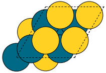
Fig 1. Clean AuPd surface |
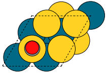
Fig 2. CO adsorbate |
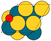
Fig 3. O adsorbate |
Here, one can also specify the rotation to change the view angle. For example, adding rotation='-90x' will save the side-view instead of the top-view of the states. One can also use the function save_pdb from the State class to save the atoms object in proteindatabank (pdb) format, as shown below for the Pd111 system:
for s in sim_system_Pd.snames:
    if sim_system_Pd.states[s].state_type != 'TS':
        sim_system_Pd.states[s].save_pdb(path='figures/Pd111/')
These files can then be editted/viewed using another program such as Avogadro or VMD.
Running simulations
The preset function run_temperatures can be used to integrate the ODEs for a range of temperatures. Here, we will use pandas to read in the saved output file for the outlet pressures from the reactor and then compute the CO conversion achieved for each temperature. Finally, we will use the preset function plot_data_simple to compare the results for each system:
from pycatkin.functions.load_input import read_from_input_file
from pycatkin.functions.presets import run_temperatures, plot_data_simple
import os
import numpy as np
import pandas as pd

fig, ax = None, None
if not os.path.isdir('figures'):
    os.mkdir('figures')
if not os.path.isdir('outputs'):
    os.mkdir('outputs')

sim_system_Au = read_from_input_file(input_path='input_AuPd.json')
sim_system_Pd = read_from_input_file(input_path='input_Pd111.json')

temperatures = np.linspace(start=423, stop=623, num=20, endpoint=True)

for sysname, sim_system in [['AuPd', sim_system_Au], ['Pd111', sim_system_Pd]]:
    run_temperatures(sim_system=sim_system,
                     temperatures=temperatures,
                     steady_state_solve=True,
                     plot_results=False,
                     save_results=True,
                     fig_path='figures/%s/' % sysname,
                     csv_path='outputs/%s/' % sysname)

    df = pd.read_csv(filepath_or_buffer='outputs/%s/pressures_vs_temperature.csv' % sysname)

    pCOin = sim_system_Pd.params['inflow_state']['CO']
    pCOout = df['pCO (bar)'].values
    xCO = 100.0 * (1.0 - pCOout / pCOin)

    fig, ax = plot_data_simple(fig=fig,
                               ax=ax,
                               xdata=temperatures,
                               ydata=xCO,
                               xlabel='Temperature (K)',
                               ylabel='Conversion (%)',
                               label=sysname,
                               addlegend=True,
                               color='teal' if sysname == 'Pd111' else 'salmon',
                               fig_path='figures/',
                               fig_name='conversion')
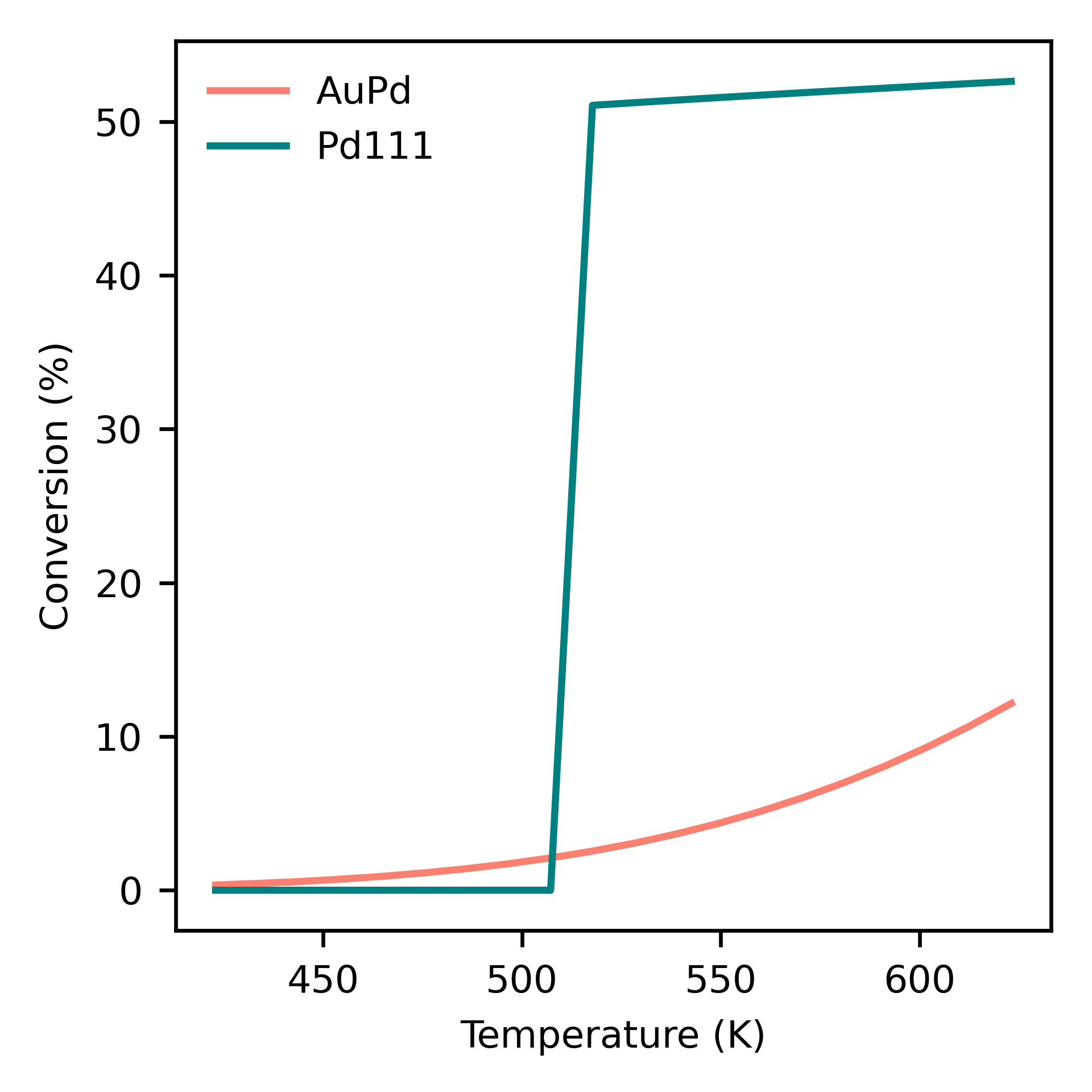
Dependence of conversion on temperature for each model system: neat Pd (Pd111) and AuPd alloy (AuPd).
- 1
Tiburski, et al. ACS Nano 15, 7, 11535, 2021. doi: 10.1021/acsnano.1c01537.
- 2
Falsig, et al. Angew. Chem. Int. Edit. 47, 4835, 2008. doi: 10.1002/anie.200801479.